Author @HiHarshSinghal
About
This BigQuery cookbook takes some interesting public datasets and presents queries you can try out using Google Colab. I also include Python code snippets to plot results of the queries for some examples. This is a work in progress and I will add queries from time to time.
Setup
Go to https://colab.research.google.com/notebooks/bigquery.ipynb to setup Colab and your access to BigQuery.
Bitcoin Transactions
The table we will query is bigquery-public-data.crypto_bitcoin.transactions and is partitioned by block_timestamp_month field. The schema of this dataset is reproduced below.
| Field name | Type | Mode | Description |
|---|---|---|---|
hash |
STRING |
REQUIRED |
The hash of this transaction |
size |
INTEGER |
NULLABLE |
The size of this transaction in bytes |
virtual_size |
INTEGER |
NULLABLE |
The virtual transaction size (differs from size for witness transactions) |
version |
INTEGER |
NULLABLE |
Protocol version specified in block which contained this transaction |
lock_time |
INTEGER |
NULLABLE |
Earliest time that miners can include the transaction in their hashing of the Merkle root to attach it in the latest block of the blockchain |
block_hash |
STRING |
REQUIRED |
Hash of the block which contains this transaction |
block_number |
INTEGER |
REQUIRED |
Number of the block which contains this transaction |
block_timestamp |
TIMESTAMP |
REQUIRED |
Timestamp of the block which contains this transaction |
block_timestamp_month |
DATE |
REQUIRED |
Month of the block which contains this transaction |
input_count |
INTEGER |
NULLABLE |
The number of inputs in the transaction |
output_count |
INTEGER |
NULLABLE |
The number of outputs in the transaction |
input_value |
NUMERIC |
NULLABLE |
Total value of inputs in the transaction |
output_value |
NUMERIC |
NULLABLE |
Total value of outputs in the transaction |
is_coinbase |
BOOLEAN |
NULLABLE |
true if this transaction is a coinbase transaction |
fee |
NUMERIC |
NULLABLE |
The fee paid by this transaction |
inputs |
RECORD |
REPEATED |
Transaction inputs |
inputs. index |
INTEGER |
REQUIRED |
0-indexed number of an input within a transaction |
inputs. spent_transaction_hash |
STRING |
NULLABLE |
The hash of the transaction which contains the output that this input spends |
inputs. spent_output_index |
INTEGER |
NULLABLE |
The index of the output this input spends |
inputs. script_asm |
STRING |
NULLABLE |
Symbolic representation of the bitcoin’s script language op-codes |
inputs. script_hex |
STRING |
NULLABLE |
Hexadecimal representation of the bitcoin’s script language op-codes |
inputs. sequence |
INTEGER |
NULLABLE |
A number intended to allow unconfirmed time-locked transactions to be updated before being finalized; not currently used except to disable locktime in a transaction |
inputs. required_signatures |
INTEGER |
NULLABLE |
The number of signatures required to authorize the spent output |
inputs. type |
STRING |
NULLABLE |
The address type of the spent output |
inputs. addresses |
STRING |
REPEATED |
Addresses which own the spent output |
inputs. value |
NUMERIC |
NULLABLE |
The value in base currency attached to the spent output |
outputs |
RECORD |
REPEATED |
Transaction outputs |
outputs. index |
INTEGER |
REQUIRED |
0-indexed number of an output within a transaction used by a later transaction to refer to that specific output |
outputs. script_asm |
STRING |
NULLABLE |
Symbolic representation of the bitcoin’s script language op-codes |
outputs. script_hex |
STRING |
NULLABLE |
Hexadecimal representation of the bitcoin’s script language op-codes |
outputs. required_signatures |
INTEGER |
NULLABLE |
The number of signatures required to authorize spending of this output |
outputs. type |
STRING |
NULLABLE |
The address type of the output |
outputs. addresses |
STRING |
REPEATED |
Addresses which own this output |
outputs. value |
NUMERIC |
NULLABLE |
The value in base currency attached to this output |
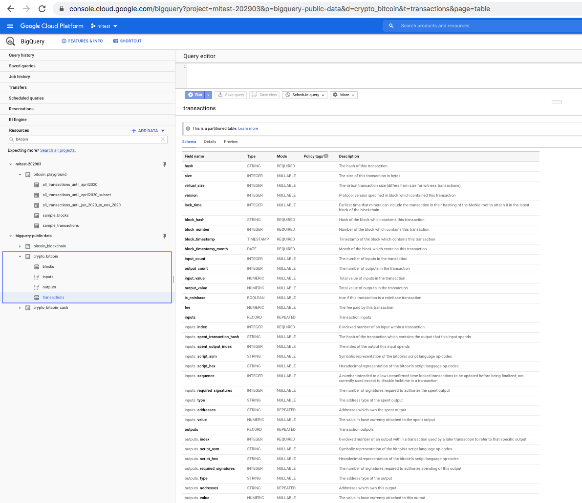
The screenshot below shows the dataset bigquery-public-data.crypto_bitcoin.transactions as it appears in the public datasets catalog.
Head over to this guide that goes into more details about Bitcoin transactions if you would like a refresher.
Selecting Bitcoin transactions and preparing a dataset for further analysis
Selecting a random collection of rows allows you to figure out general trends in your data without having to analyze the entire dataset. Below, we will create a table and populate it with a random selection of bitcoin transactions.
create table `mltest-202903.bitcoin_playground.sample_transactions`  as (1)
select
    *
from
    `bigquery-public-data.crypto_bitcoin.transactions` (2)
where
    block_timestamp_month = '2020-05-01' (3)
    and rand() <= 0.01 (4)
;| 1 | The name of the table created is composed of project name.dataset name.table name where the project name is mltest-202903, the dataset name is bitcoin_playground and the table name is sample_transactions. |
| 2 | The name of the public dataset table from which to read the Bitcoin transactions data. |
| 3 | Table is partitioned on the block_timestamp_month column and we are filtering for 2020-05-01. |
| 4 | rand() returns a random value between (0, 1]. We filter for random values ⇐ 0.01. This should samples 1% of rows from the table. |
The table created is approximately 80 MB in size.
You can run the query in Google Colab (screenshot below)
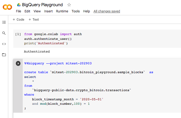
Another way to select a random subset is to extract blocks so you get all the transactions inside of the block. This is useful if you want to analyze mining fees and need to look at all the transactions inside the block.
create table `mltest-202903.bitcoin_playground.sample_blocks`  as
select
    *
from
    `bigquery-public-data.crypto_bitcoin.transactions`
where
    block_timestamp_month = '2020-05-01'
    and mod(block_number,100) = 1 (1)
;| 1 | MOD(a, b) returns the remainder of the division of a by b. In this case, we divide block_number by 100 and check if the remainder is 1. This should sample 1% of the blocks. You can choose to use any number between 0 and 99 in place of 1 in mod(block_number,100) = 1 and you should sample 1% of the blocks. The underlying assumption is that block numbers are incremented uniformly. |
The table created is approximately 93 MB in size.
We will create a dataset of a few columns that will be utilized for further analyses into transactions growth and fees.
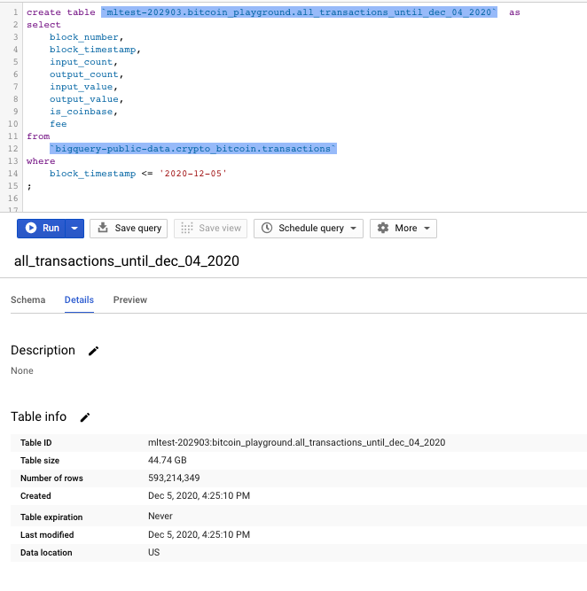
create table `mltest-202903.bitcoin_playground.all_transactions_until_dec_04_2020`  as
select
    block_number,
    block_timestamp,
    input_count,
    output_count,
    input_value,
    output_value,
    is_coinbase,
    fee
from
    `bigquery-public-data.crypto_bitcoin.transactions`
where
    block_timestamp <= '2020-12-05'
;
The dataset created is approximately 44 GB in size.
Schema of the table created above.
| Field name | Type | Mode | Description |
|---|---|---|---|
block_number |
INTEGER |
REQUIRED |
Number of the block which contains this transaction |
block_timestamp |
TIMESTAMP |
REQUIRED |
Timestamp of the block which contains this transaction |
input_count |
INTEGER |
NULLABLE |
The number of inputs in the transaction |
output_count |
INTEGER |
NULLABLE |
The number of outputs in the transaction |
input_value |
NUMERIC |
NULLABLE |
Total value of inputs in the transaction |
output_value |
NUMERIC |
NULLABLE |
Total value of outputs in the transaction |
is_coinbase |
BOOLEAN |
NULLABLE |
true if this transaction is a coinbase transaction |
fee |
NUMERIC |
NULLABLE |
The fee paid by this transaction |
Run the query below if you would like to drop the table.
drop table if exists `mltest-202903.bitcoin_playground.all_transactions_until_dec_04_2020`;Transactions per block
The number of transactions per block has been steadily increasing but is bound by the scalability problem. Lets analyze transactions per block and quantify the number of blocks by the transactions they contain.
with hash_ct_by_block_num as ( (1)
  select
    block_number,
    count(*) as per_block_transaction_hash_ct
  from `mltest-202903.bitcoin_playground.all_transactions_until_dec_04_2020`
  group by
    block_number
)
select
  floor(per_block_transaction_hash_ct/100) as bkt_100, (2)
  count(distinct block_number) as block_ct
from hash_ct_by_block_num (3)
group by
  bkt_100
order by
  bkt_100
;| 1 | CTE to aggregate count of transactions by block_number. Common Table Expression (CTE) are very useful when writing complex queries. Think of them as creating tables on fly that you can use in later sections of the same query. Pretty neat! |
| 2 | Bucket the number of transactions by each block in buckets of size 100. For e.g., if per_block_transaction_hash_ct is 50, floor(50/100) will be 0. The function floor rounds down to the nearest integer. The result of floor(per_block_transaction_hash_ct/100) if 0 identifies the bucket [1, 99], 1 identifies [100, 199], 2 identifies [200, 299] and so on. |
| 3 | Reference the CTE query name hash_ct_by_block_num which acts like a temporary table name. |
The Python snippet below can be used to visualize the distribution of the number of blocks for each transaction count bucket.
# function to create string label for the buckets
def create_label(val, bucket_width=100):
    return "[" + str(int(val)*bucket_width) + ',' + str((int(val)*bucket_width)+(bucket_width-1)) + "]"

df_hash_per_block['bkt_100_label'] = df_hash_per_block['bkt_100'].map(create_label) (1)| 1 | df_hash_per_block is the pandas dataframe that contains the results of the preceding query. We also create an additional column,bkt_100_label to use as labels for better readability in the plot. |
Lets plot the distribution of number of blocks against the number of transactions per block.
import plotly.express as px

fig = px.bar(df_hash_per_block,
  x='bkt_100_label',
  y='block_ct')

fig.show()
This is what the Colab cells look like for the above.
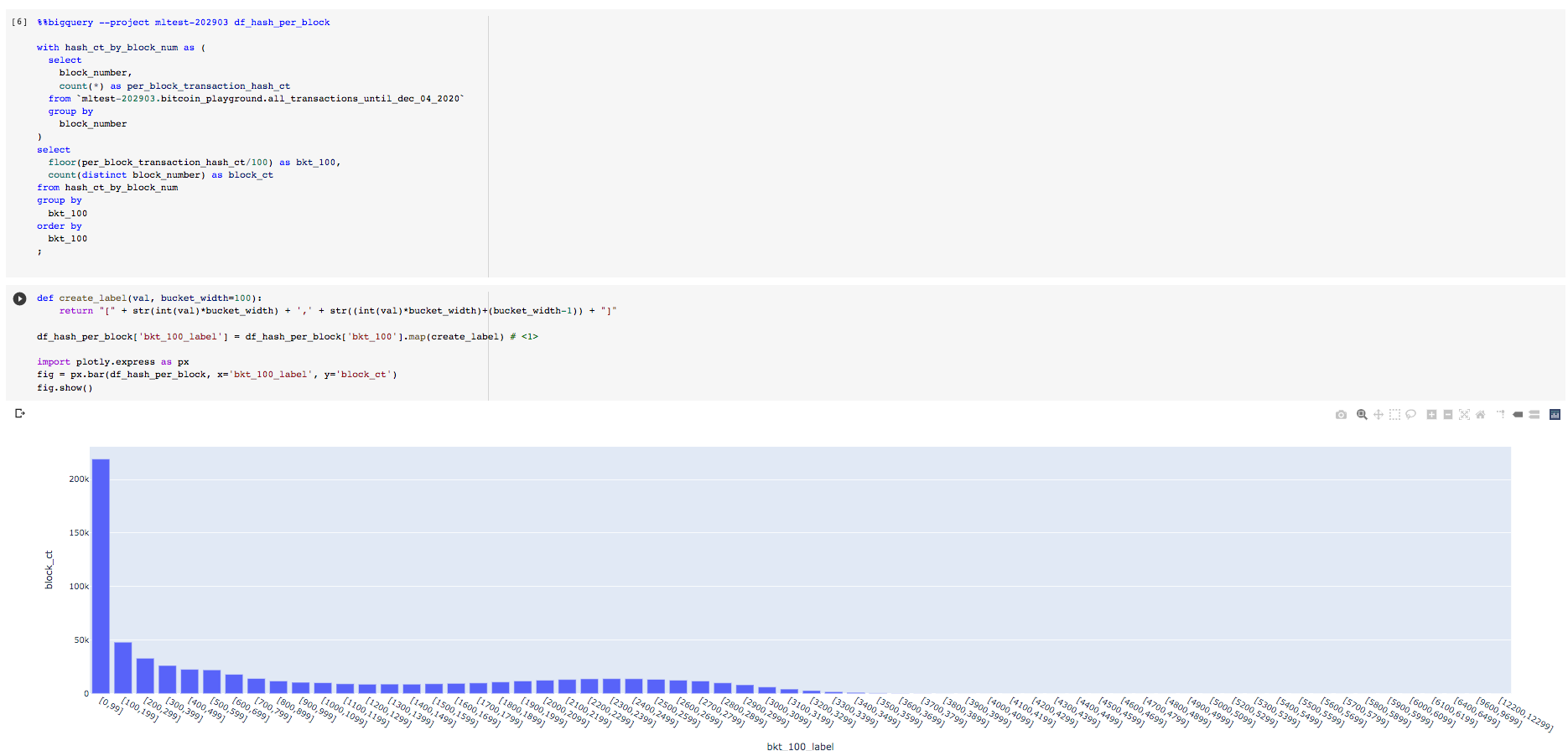
Seems like the vast majority of blocks have < 100 transactions.
Given the rise in popularity of Bitcoin and increase in hash power, the number of transactions per block has been steadily rising. We will now look at the average transactions per block over the years.
with hash_ct_by_block_num as (
  select
    extract(year from block_timestamp) as block_timestamp_year, (1)
    block_number,
    count(*) as per_block_transaction_hash_ct
  from `mltest-202903.bitcoin_playground.all_transactions_until_dec_04_2020`
  group by
    block_timestamp_year,
    block_number
)
select
  block_timestamp_year,
  avg(per_block_transaction_hash_ct) as avg_per_block_transaction_hash_ct (2)
from hash_ct_by_block_num
group by
  block_timestamp_year
order by
  block_timestamp_year
;| 1 | extract is a Timestamp function that can extract certain parts of a timestamp such as the year, month, day and so on. |
| 2 | avg is an Aggregate function. |
Plot the results using the snippet below.
import plotly.express as px
fig = px.line(df_hash_per_block,
    x="block_timestamp_year",
    y="avg_per_block_transaction_hash_ct",
    title="Average transactions per block across the years")
fig.show()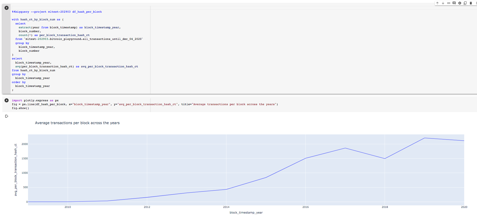
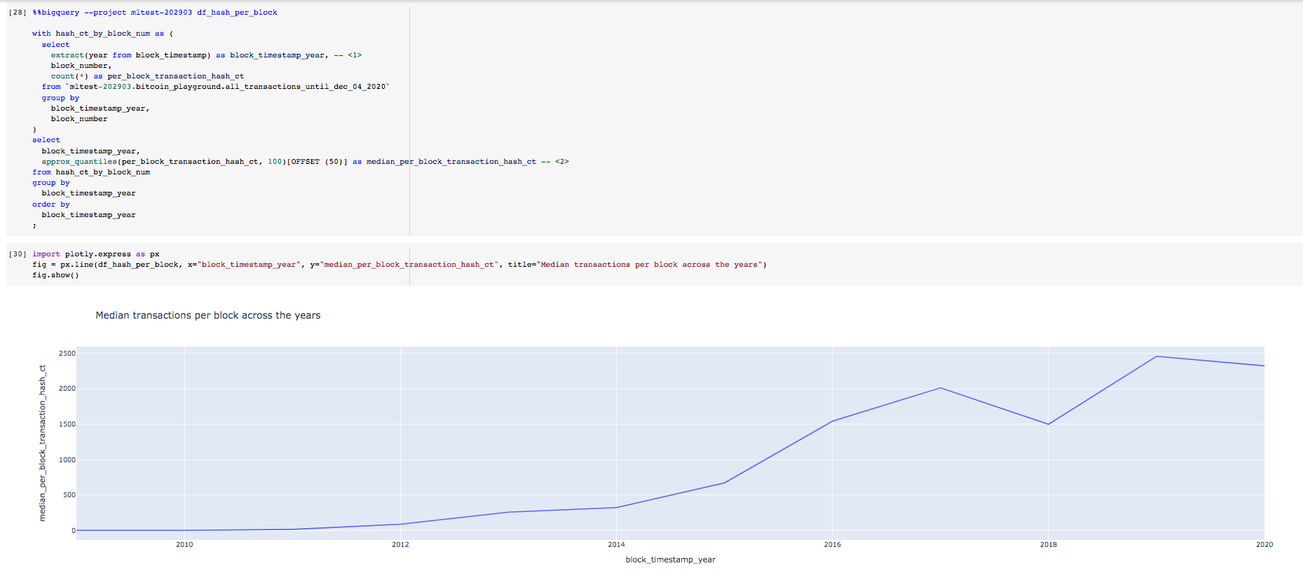
The average transactions per block has been steadily increasing. Lets also check the median number of transactions per block across the years since average can be influenced by very large numbers.
median requires ordering the data and can be a very expensive operation when dealing with very large amounts of data. In BigQuery, the median is computed using Approximate Aggregate function, APPROX_QUANTILES.
with hash_ct_by_block_num as (
  select
    extract(year from block_timestamp) as block_timestamp_year, (1)
    block_number,
    count(*) as per_block_transaction_hash_ct
  from `mltest-202903.bitcoin_playground.all_transactions_until_dec_04_2020`
  group by
    block_timestamp_year,
    block_number
)
select
  block_timestamp_year,
  approx_quantiles(per_block_transaction_hash_ct, 100)[OFFSET (50)] as median_per_block_transaction_hash_ct (2)
from hash_ct_by_block_num
group by
  block_timestamp_year
order by
  block_timestamp_year
;| 1 | extract is a Timestamp function that can extract certain parts of a timestamp such as the year, month, day and so on. |
| 2 | approx_quantiles is an Approximate Aggregate function. The way this function works is that it returns an array of number + 1 elements where the first element is the approximate minimum and the last element is the approximate maximum. Using the array function offset you can extract the specific percentile value you desire by indexing the array returned by approx_quantiles. |
Plot the results using the snippet below.
import plotly.express as px
fig = px.line(df_hash_per_block,
  x="block_timestamp_year",
  y="median_per_block_transaction_hash_ct",
  title="Median transactions per block across the years")
fig.show()
This is the result of the above query and Python snippet. The average and the median follow a similar trend. Eyeballing the values does not show any large deviations.
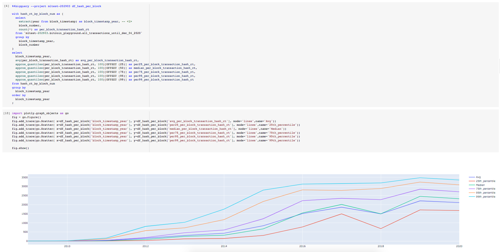
Lets write a query to extract the average, median and other order statistics.
with hash_ct_by_block_num as (
  select
    extract(year from block_timestamp) as block_timestamp_year, (1)
    block_number,
    count(*) as per_block_transaction_hash_ct
  from `mltest-202903.bitcoin_playground.all_transactions_until_dec_04_2020`
  group by
    block_timestamp_year,
    block_number
)
select
  block_timestamp_year,
  avg(per_block_transaction_hash_ct) as avg_per_block_transaction_hash_ct,
-- Extract ordered statistics
  approx_quantiles(per_block_transaction_hash_ct, 100)[OFFSET (25)] as per_25_per_block_transaction_hash_ct,
  approx_quantiles(per_block_transaction_hash_ct, 100)[OFFSET (50)] as median_per_block_transaction_hash_ct,
  approx_quantiles(per_block_transaction_hash_ct, 100)[OFFSET (75)] as per_75_per_block_transaction_hash_ct,
  approx_quantiles(per_block_transaction_hash_ct, 100)[OFFSET (95)] as per_95_per_block_transaction_hash_ct,
  approx_quantiles(per_block_transaction_hash_ct, 100)[OFFSET (99)] as per_99_per_block_transaction_hash_ct
from hash_ct_by_block_num
group by
  block_timestamp_year
order by
  block_timestamp_year
;
Plot using the snippet below.
import plotly.graph_objects as go

fig = go.Figure()

fig.add_trace(go.Scatter(
  x=df_hash_per_block['block_timestamp_year'],
  y=df_hash_per_block['avg_per_block_transaction_hash_ct'],
  mode='lines',
  name='Avg')
  )
fig.add_trace(go.Scatter(
  x=df_hash_per_block['block_timestamp_year'],
  y=df_hash_per_block['per25_per_block_transaction_hash_ct'],
  mode='lines',
  name='25th_percentile')
  )
fig.add_trace(go.Scatter(
  x=df_hash_per_block['block_timestamp_year'],
  y=df_hash_per_block['median_per_block_transaction_hash_ct'],
  mode='lines',
  name='Median')
  )
fig.add_trace(go.Scatter(
  x=df_hash_per_block['block_timestamp_year'],
  y=df_hash_per_block['per75_per_block_transaction_hash_ct'],
  mode='lines',
  name='75th_percentile')
  )
fig.add_trace(go.Scatter(
  x=df_hash_per_block['block_timestamp_year'],
  y=df_hash_per_block['per95_per_block_transaction_hash_ct'],
  mode='lines',
  name='95th_percentile')
  )
fig.add_trace(go.Scatter(
  x=df_hash_per_block['block_timestamp_year'],
  y=df_hash_per_block['per99_per_block_transaction_hash_ct'],
  mode='lines',
  name='99th_percentile')
  )

fig.show()
The screenshot below show the Colab cells for the above.
You can also loop through the y variables as shown in the snippet below to produce the plot.
import plotly.graph_objects as go

y_vars = ['avg_per_block_transaction_hash_ct',
'per25_per_block_transaction_hash_ct', 'median_per_block_transaction_hash_ct',
'per75_per_block_transaction_hash_ct', 'per95_per_block_transaction_hash_ct',
'per99_per_block_transaction_hash_ct']

fig = go.Figure()

for y_var in y_vars:
  fig.add_trace(go.Scatter(
    x=df_hash_per_block['block_timestamp_year'],
    y=df_hash_per_block[y_var],
    mode='lines',
    name=y_var.split('_')[0]
  ))

# Figure titles
fig.update_layout(
    title="Statistics related of transactions per block",
    xaxis_title="Year",
    yaxis_title="Transactions per block"
)

fig.show()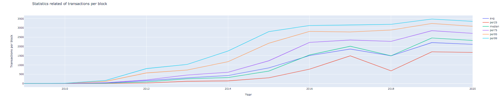
Transactions Growth
The number of transactions over the years has been steadily increasing. Lets quantify the daily transactions count and plot it.
select
    date(block_timestamp) as block_timestamp_date,
    count(*) as ct_transactions
  from `mltest-202903.bitcoin_playground.all_transactions_until_dec_04_2020`
  group by
    block_timestamp_date
order by
  block_timestamp_date
;
Plot the daily transactions count.
import plotly.express as px

fig = px.line(df_hash_per_block,
    x="block_timestamp_date",
    y="ct_transactions",
    title="Daily Transactions")

fig.show()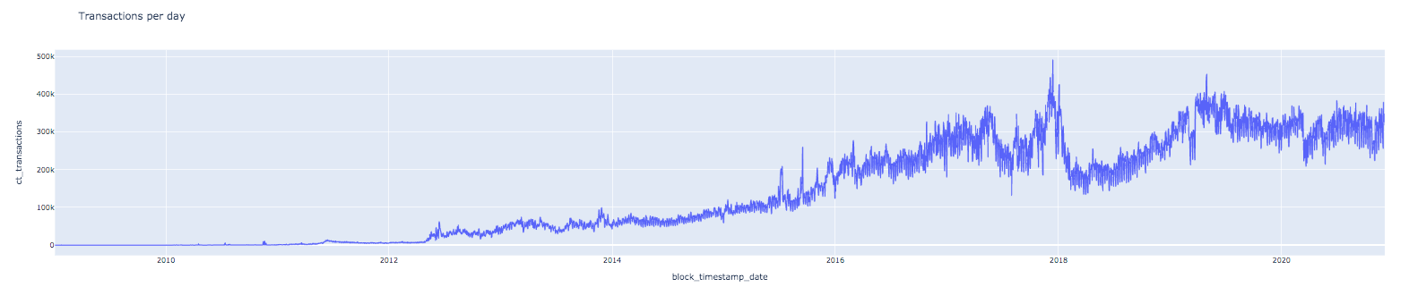
Lets compute a moving average of the transactions count to smooth out some of the daily variations. The query below will show you how to compute a 7-day moving average.
with daily_transactions as (
    select
      date(block_timestamp) as block_timestamp_date,
      count(*) as ct_transactions
    from `mltest-202903.bitcoin_playground.all_transactions_until_dec_04_2020`
    group by
      block_timestamp_date
)
select
  block_timestamp_date,
  ct_transactions,
  AVG(ct_transactions) (1)
    OVER ( (2)
      ORDER BY block_timestamp_date (3)
      ROWS BETWEEN 6 PRECEDING AND CURRENT ROW (4)
    ) as ma_7d_transactions
from
  daily_transactions
order by
  block_timestamp_date
;| 1 | Example of an aggregate analytic function. |
| 2 | The over clause defines the window of rows over which the aggregate function, avg in this case will be computed. |
| 3 | The rows are ordered by the block_timestamp_date column. |
| 4 | We are looking to compute a 7-day moving average so we include the current row along with the 6 previous rows. |
import plotly.graph_objects as go

fig = go.Figure()

fig.add_trace(go.Scatter(
  x=df_transactions_daily['block_timestamp_date'],
  y=df_transactions_daily['ct_transactions'],
  mode='lines',
  name='Daily Transactions Count')
  )
fig.add_trace(go.Scatter(
  x=df_transactions_daily['block_timestamp_date'],
  y=df_transactions_daily['ma_7d_transactions'],
  mode='lines',
  name='7-day Moving Average of Daily Transactions Count')
  )

fig.update_layout(
    title="Daily Transactions Count",
    xaxis_title="Date",
    yaxis_title="Transactions/day"
)

fig.show()
We will now look at the BTC to USD price movement in relation to daily transactions. I’ve downloaded historical daily BTC/USD data on the Coinbase Gemini exchange from here.
I uploaded the CSV file into Google Sheets and created a table in BigQuery from this spreadhseet. See instructions on how this can be done here.
The query below combines the computation to quantify daily transactions count, 7-day moving average of daily transactions count and joins with open USD price of 1 BTC on Coinbase exchange.
with daily_transactions as (
    select
      date(block_timestamp) as block_timestamp_date,
      count(*) as ct_transactions
    from `mltest-202903.bitcoin_playground.all_transactions_until_dec_04_2020`
    group by
      block_timestamp_date
),
moving_avg_d as (
    select
      block_timestamp_date,
      ct_transactions,
      AVG(ct_transactions)
        OVER (
          ORDER BY block_timestamp_date
          ROWS BETWEEN 6 PRECEDING AND CURRENT ROW
        ) as ma_7d_transactions
    from
      daily_transactions
    order by
      block_timestamp_date
),
daily_usd_per_btc as (
    select
      date(`date`) as date_val, (1)
      `open` as usd_open
    from `mltest-202903.bitcoin_playground.btc_to_usd`
)
select
  a.date_val,
  a.usd_open,
  b.ct_transactions,
  b.ma_7d_transactions
from daily_usd_per_btc a
join moving_avg_d b on (a.date_val = b.block_timestamp_date)
;| 1 | Using backticks since the column name is a reserved word. You can also change the original spreadhseet column name to avoid the confusion or the need for backticks. |
Plot using the snippet below.
import plotly.graph_objects as go
from plotly.subplots import make_subplots

# Create figure with secondary y-axis
fig = make_subplots(specs=[[{"secondary_y": True}]])

fig.add_trace(go.Scatter(
  x=df_transactions_daily['date_val'],
  y=df_transactions_daily['ct_transactions'],
  mode='lines',
  name='Daily Transactions Count')
  )
fig.add_trace(go.Scatter(
  x=df_transactions_daily['date_val'],
  y=df_transactions_daily['ma_7d_transactions'],
  mode='lines',
  name='7-day Moving Average')
  )

fig.add_trace(go.Scatter(
  x=df_transactions_daily['date_val'],
  y=df_transactions_daily['usd_open'],
  mode='lines',
  name='USD Open Price of 1 BTC'
  ),
  secondary_y = True
  )


# Figure title
fig.update_layout(
    title_text="Daily Transactions and Open Price of 1 BTC in USD"
)

# Set x-axis title
fig.update_xaxes(title_text="Date")

# Set y-axes titles
fig.update_yaxes(title_text="Transactions/day", secondary_y=False)
fig.update_yaxes(title_text="Open Price in USD of 1 BTC", secondary_y=True)

# Horizontal legend layout and move below the plotting area
fig.update_layout(legend=dict(
    orientation="h",
    yanchor="top",
    y=-0.15,
    xanchor="left",
    x=0.3
))

fig.show()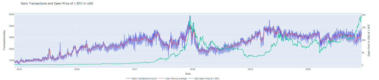
Growth in Daily Input Addresses
Analyzing growth in input addresses.
with base_data as (  (1)
    select
        date(block_timestamp) as block_timestamp_date,
        input_data.addresses as input_data_addresses
    from
        `bigquery-public-data.crypto_bitcoin.transactions`
    CROSS JOIN UNNEST(inputs) as input_data
    where
        block_timestamp_month >= '2015-01-01'
),
individual_input_address as ( (2)
    select
        block_timestamp_date,
        input_address
    from base_data
    CROSS JOIN UNNEST(input_data_addresses) as input_address
),
dist_input_addresses_per_day as ( (3)
    select
        block_timestamp_date,
        count(distinct input_address) as distinct_input_addresses
    from individual_input_address
    group by
        block_timestamp_date
    order by
        block_timestamp_date
),
moving_avg_d as ( (4)
    select
        block_timestamp_date,
        distinct_input_addresses,
        AVG(distinct_input_addresses)
        OVER (
            ORDER BY block_timestamp_date
            ROWS BETWEEN 6 PRECEDING AND CURRENT ROW
        ) as ma_7d_input_addresses,
        AVG(distinct_input_addresses)
        OVER (
            ORDER BY block_timestamp_date
            ROWS BETWEEN 29 PRECEDING AND CURRENT ROW
      ) as ma_30d_input_addresses
    from
        dist_input_addresses_per_day
),
daily_usd_per_btc as ( (5)
    select
        date(`date`) as date_val,
        `open` as usd_open
    from `mltest-202903.bitcoin_playground.btc_to_usd`
)
select
    a.block_timestamp_date,
    a.distinct_input_addresses,
    a.ma_7d_input_addresses,
    a.ma_30d_input_addresses,
    b.usd_open
from moving_avg_d a
join daily_usd_per_btc b on (a.block_timestamp_date = b.date_val)
order by
   block_timestamp_date
;| 1 | Extract the addresses array from the inputs column. |
| 2 | Extract each individual input addresses. |
| 3 | Count the distinct number of input addresses by day. |
| 4 | Compute moving averages. |
| 5 | Select the daily USD open price of 1 BTC. |
Plot the daily input addresses count with the USD open price of 1 BTC
import plotly.graph_objects as go
from plotly.subplots import make_subplots

fig = make_subplots(specs=[[{"secondary_y": True}]])
fig.add_trace(go.Scatter( x=df['block_timestamp_date'], y=df['distinct_input_addresses'], mode='lines',name='Daily'))
fig.add_trace(go.Scatter( x=df['block_timestamp_date'], y=df['ma_7d_input_addresses'], mode='lines',name='7d MA'))
fig.add_trace(go.Scatter( x=df['block_timestamp_date'], y=df['ma_30d_input_addresses'], mode='lines',name='30d MA'))
fig.add_trace(go.Scatter( x=df['block_timestamp_date'], y=df['usd_open'], mode='lines',name='USD Open Price of 1 BTC'), secondary_y = True)

# Figure title
fig.update_layout(
    title_text="Daily Distinct Input Addresses and Open Price of 1 BTC in USD"
)

# Set x-axis title
fig.update_xaxes(title_text="Date")

# Set y-axes titles
fig.update_yaxes(title_text="Distinct Input Addresses/day", secondary_y=False)
fig.update_yaxes(title_text="Open Price in USD of 1 BTC", secondary_y=True)

# Horizontal legend layout and move below the plotting area
fig.update_layout(legend=dict(
    orientation="h",
    yanchor="top",
    y=-0.15,
    xanchor="left",
    x=0.3
))

fig.show()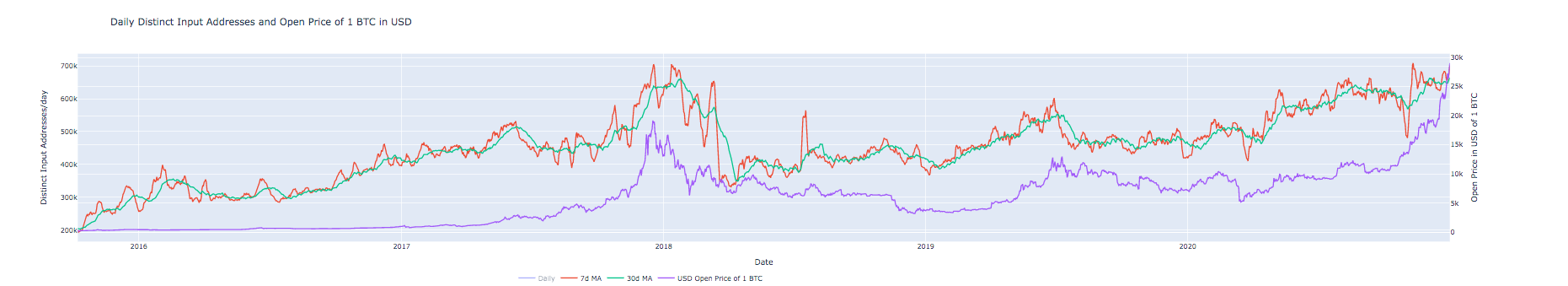
Here is the Colab notebook if you would like to reproduce the analysis.